Coarse-Fine Volatility
Description
The coarse-fine volatility correlation is a multi-time-scale analysis of volatility.
\begin{eqnarray}
v_{c}^{\tau}(t)&=&\bigg{|}\sum_{i=1}^{\tau}{r_{t-i}}\bigg{|}\\
v_{f}^{\tau}(t)&=&\sum_{i=1}^{\tau}{|r_{t-i}|}.
\end{eqnarray}
While the coarse volatility is the absolute value of the price movement in \(\tau\) days, the fine volatility is the sum of the absolute price return in \(\tau\) days. \(\tau=5\) is starndard as it stands for day-week time-scales.
\begin{equation}
\rho_{cf}^{\tau}(k)=Corr(v_{c}^{\tau}(t+k),v_{f}^{\tau}(t)).
\end{equation}
[Muller_1997][Gavrishchaka_2003] reported that there exists the negative asymmetry of the lead-lag correlation quantified by the difference
\begin{equation}
\Delta\rho_{cf}^{\tau}(k)=\rho_{cf}^{\tau}(k)-\rho_{cf}^{\tau}(-k).
\end{equation}
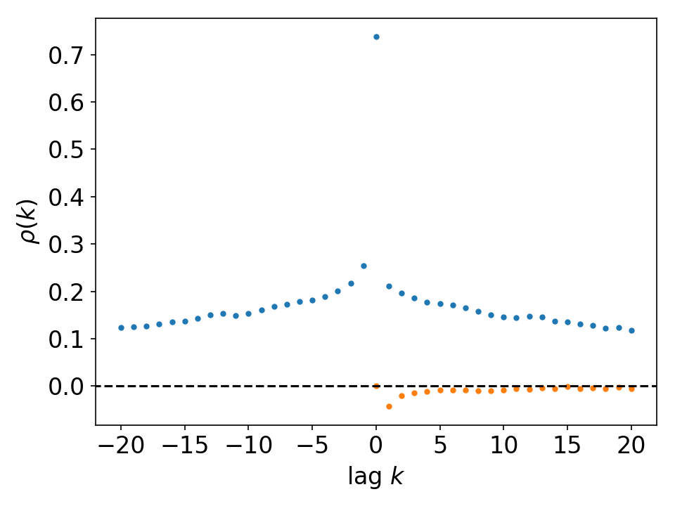
Fig. Averaged result for S&P500 firms daily price return
Code Example
import datetime as dt
import pandas_datareader.data as web
import numpy as np
import stylefact.finance as sff
import stylefact.visualize as sfv
st = dt.datetime(1990,1,1)
en = dt.datetime(2020,1,1)
data = web.get_data_yahoo('GM', start=st, end=en)
prices = data['Adj Close'].to_numpy()
log_prices = np.log(prices)
returns = np.diff(log_prices)
x,y = sff.coarsefine_volatility(returns)
sfv.coarsefine_volatility(x,y,'coarsefine')
References
| [GG03] | V. V. Gavrishchaka and S. B. Ganguli. Volatility forecasting from multiscale and high-dimensional market data. Neurocomputing, 55(1):285–305, 2003. |
| [MDD+97] | Ulrich A. Müller, Michel M. Dacorogna, Rakhal D. Davé, Richard B. Olsen, Olivier V. Pictet, and Jacob E. von Weizsäcker. Volatilities of different time resolutions - analyzing the dynamics of market components. Journal of Empirical Finance, 4(2):213–239, 1997. |